Data structures & algorithms

Section links stay in this document. Blue topic links open separate readers. Historical writing, editorial corrections and AI-assisted study additions are distinguished in the text. Numbering follows this reader’s order; historical claims still need review.

1 Self-taught DSA and LeetCode problem-solving patterns – study additions

AI-assisted editorial study additions: original explanations and illustrations, not verbatim historical writing nor a transcript. This is explicitly self-taught data structures and algorithms study, including LeetCode-style practice, not a claim of enrolment in a computer-science or SYDE DSA course.

1.1 Choose a representation before an algorithm

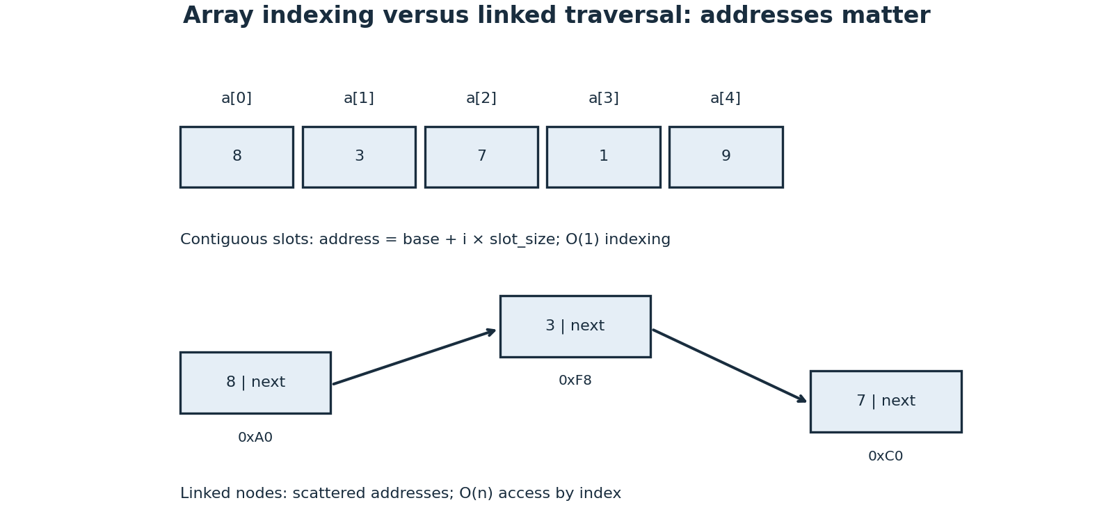
An abstract data type specifies permitted operations; a data structure implements them. An array supports constant-time indexing with contiguous slots, but insertion near the front shifts elements. A dynamic array has amortized constant-time append, although an individual resizing append is linear. A linked list has constant-time local insertion when the relevant node or predecessor is already known, but finding that location can cost linear time. Pointer overhead and cache locality matter in practice; equal asymptotic bounds do not imply equal performance.

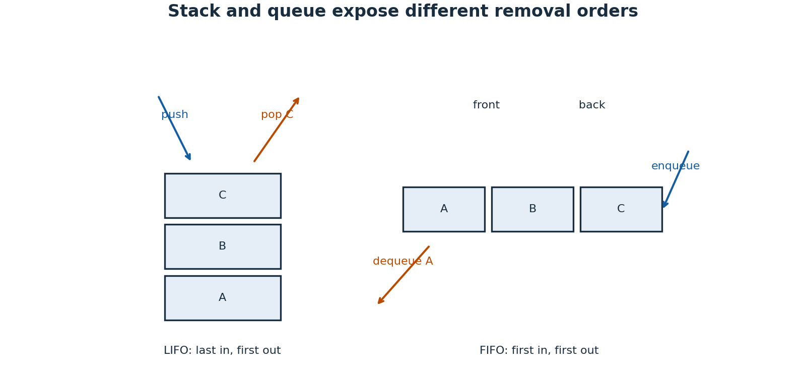
Array slots have arithmetic addresses, while linked nodes require pointer traversal. Addresses and slot sizes are schematic; language runtimes may store references to objects rather than the objects themselves in array slots.

A stack removes the most recently added item and naturally models nested work. A queue removes the earliest item and supports breadth-first exploration. Implement queue removal without shifting an entire array, for example using a ring buffer or deque. Hash tables offer expected constant-time lookup under suitable hashing and load assumptions; collision-heavy worst cases may be linear. A key must obey the container’s equality and hash contract, and mutating a hash-relevant key while stored can break lookup.

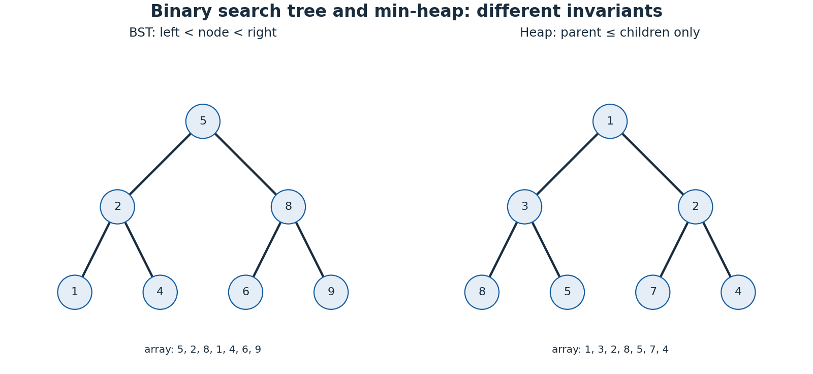
After inserting A, B, then C, a stack removes C while a queue removes A. Arrows identify logical operations, not a required physical memory arrangement.

A binary search tree orders entire subtrees, not just immediate children. Search costs \(O(h)\) with height \(h\); balance is what makes that logarithmic. A binary heap maintains parent–child priority and completeness but does not globally sort siblings. A min-heap gives \(O(1)\) minimum access, \(O(\log n)\) insertion/removal, and \(O(n)\) bottom-up construction. In a zero-based array, children are \(2i+1\) and \(2i+2\). A heap is ideal for repeated best-next extraction, not arbitrary membership search.

The search tree orders left and right subtrees; the min-heap orders only ancestors relative to descendants. Arrays below show level-order layouts, which are not sorted sequences. Keys are distinct in this example.

1.2 Complexity is a claim with a cost model

Big-O gives an asymptotic upper bound; Big-Theta gives a tight growth class. Specify input size, operation cost, auxiliary storage, recursion depth, and whether the claim is worst-case, expected, or amortized. Expected analysis averages over a stated randomness model; amortized analysis distributes cost over an operation sequence without requiring randomness. Sorting huge integers or comparing long strings changes the cost model. Outputting all subsets already requires exponential output, regardless of clever bookkeeping.

1.3 Graphs, dependencies, and connectivity

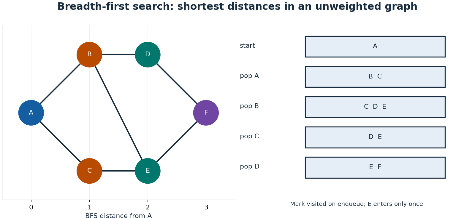
An adjacency list uses \(O(V+E)\) storage for a sparse graph. BFS with a FIFO queue finds fewest-edge distances in an unweighted graph. Mark a vertex when enqueued, and save its predecessor once; this prevents duplicate frontier growth and reconstructs a shortest path. DFS uses a stack or recursion and is useful for reachability, cycle reasoning, and finishing order, but does not generally find a shortest path. Both take \(O(V+E)\) with adjacency lists and constant-time visited checks.

BFS layers and queue snapshots for a connected unweighted undirected graph. Alphabetical neighbour order is assumed; another tie order changes the tree but not the distances.

Dijkstra’s algorithm repeatedly settles the smallest tentative distance and relaxes outgoing edges. Its correctness requires nonnegative edge weights; a negative edge can improve an already settled vertex. With a heap, skip stale distance entries rather than processing them as new discoveries. Bellman–Ford handles negative edges and detects reachable negative cycles; finite shortest paths fail when such cycles can influence the destination.

Topological order exists only for a directed acyclic graph. Kahn’s method repeatedly removes indegree-zero vertices; processing fewer than \(V\) reveals a cycle. DFS reverse finishing order also works when cycles are correctly detected. Union–find answers incremental undirected connectivity: union by rank or size plus path compression gives near-constant amortized cost \(O(\alpha(n))\). It is not a path-finding algorithm and does not by itself support arbitrary edge deletion.

1.4 Binary search is an invariant, not a remembered template

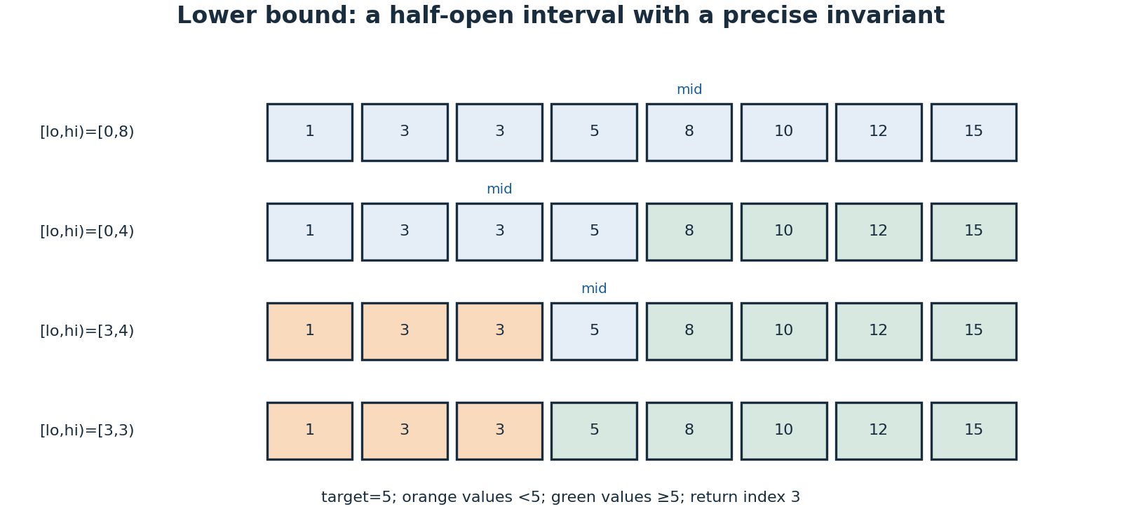
For sorted \(a\), lower bound seeks the first index whose value is at least target \(t\). Maintain a half-open unresolved interval \([lo,hi)\), with all indices below \(lo\) known smaller than \(t\) and all indices at or above \(hi\) known at least \(t\). Initially \(lo=0\), \(hi=n\), so both outside assertions are vacuous.

While \(lo<hi\), choose \(mid=lo+\lfloor(hi-lo)/2\rfloor\).
If \(a[mid]<t\), assign \(lo=mid+1\); otherwise assign \(hi=mid\).
Return \(lo\) when the interval is empty. The result may equal \(n\).

The interval strictly shrinks and the assertions survive each update. Empty input, duplicates, all-smaller, all-larger, and exact-boundary cases are essential tests. For binary search on an answer, first prove the feasibility predicate is monotone; numeric order alone does not guarantee that property.

A complete lower-bound trace for target five. Orange cells are proven too small, green cells are proven large enough, and the unresolved half-open interval shrinks to insertion index three.

1.5 Sorting, recursion, and optimal substructure

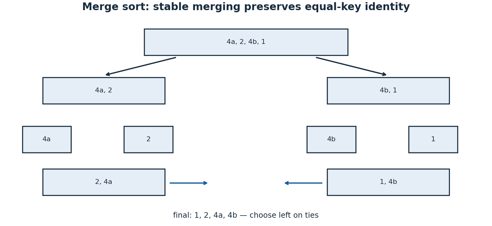
Merge sort divides, solves smaller instances, and merges sorted outputs. Taking from the left on equal keys preserves stability, meaning equal-key records retain original relative order. Standard array merge sort uses \(O(n\log n)\) time and \(O(n)\) auxiliary space. Quicksort is typically fast and expected \(O(n\log n)\) with suitable randomization, but ordinary versions have quadratic worst cases and are unstable. Heapsort offers worst-case \(O(n\log n)\) with constant auxiliary array storage but is unstable. Insertion sort is quadratic worst-case, stable with careful comparisons, and useful for small or nearly sorted inputs.

A merge-sort decomposition with equal keys labelled by original identity. The final merge takes 4a before 4b because ties choose the left input; labels are payload identity, not extra sorting keys.

Every recursive function needs a base case and a decreasing progress measure. Backtracking explores choices and undoes state before exploring siblings; copying results avoids later mutation corrupting saved answers. Memoization helps only when repeated subproblems share a sufficient state description. Dynamic programming requires a recurrence, boundary values, dependency order, and a proof that no relevant history was discarded.

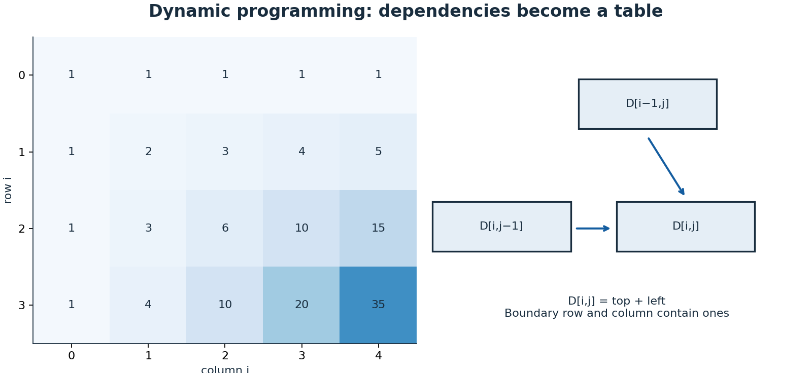
For right/down grid paths, \(D[i,j]=D[i-1,j]+D[i,j-1]\), with boundary row and column equal to one. Obstacles change the recurrence to zero at blocked cells. A row-buffer implementation uses \(O(\text{columns})\) space because only top and left are needed. Greedy decisions need an exchange argument or another correctness proof: locally attractive choices are not automatically globally optimal. Earliest finishing time solves unweighted interval scheduling; choosing the shortest interval does not generally do so.

Exact path counts for an obstacle-free four-by-five cell grid, starting at the upper-left cell. Each interior count adds the two predecessor counts; right/down motion makes the dependency graph acyclic.

1.6 Reusable patterns and falsifiable tests

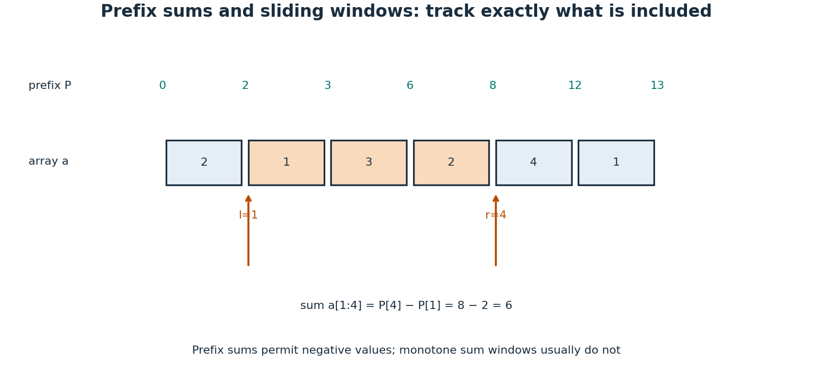
Prefix sums \(P[0]=0\), \(P[i+1]=P[i]+a[i]\) answer half-open range sums by \(P[r]-P[l]\), including negative values. A variable-length sum window usually needs nonnegative entries so extension cannot decrease the sum. For arbitrary signs, a prefix-sum frequency map can count target-sum subarrays; initialize the zero prefix count to one. Sorted two-pointer pair search relies on ordering: increasing the left endpoint raises the sum, while decreasing the right lowers it. A longest-substring-without-repeats window instead maintains frequency or last-seen invariants, not numeric monotonicity.

Prefix boundaries sit between entries; the highlighted half-open slice excludes index four. The arithmetic identity always holds, whereas a monotone sliding-window decision needs additional assumptions.

Test empty and singleton inputs, duplicate keys, negative numbers, overflow limits, disconnected graphs, cycles, unreachable targets, and deep recursion. Compare optimized solutions against brute force on small exhaustive inputs. Check properties such as sorted output preserving the input multiset, valid reconstructed paths, and heap order after every mutation. Practice should end with an explained invariant and failure case, not just an accepted submission.

1.7 Independent learning references

See MIT OpenCourseWare: Introduction to Algorithms. The Waterloo 2022/23 SYDE calendar lists DSA subject matter, but is used only as a topic comparison; this section makes no SYDE 223 completion claim.

Download original LaTeX source